One important aspect of economic scenario generators (ESG) is their ability to capture stylized facts observed in the historical data. Examples of stylized facts include but are not limited to, correlations between macroeconomic indicators, leading and lagging effects, level-dependent dynamic relationships, and even inverse relationships during stress periods.
In this blog, we present a few specific economic scenarios and discuss the behavior of macroeconomic variables we observed. The scenario examples described here are not cherry-picked but rather randomly selected from thousands of scenarios generated by our proprietary AI model.
In all illustrated economic scenarios, 2023 Q4 is the last actual period, and 2024 Q1 is the first generated period. For the purpose of this discussion, we limited the scenario examples to 4 years.
We also published examples of 2025 economic scenarios.
Recessionary Scenario
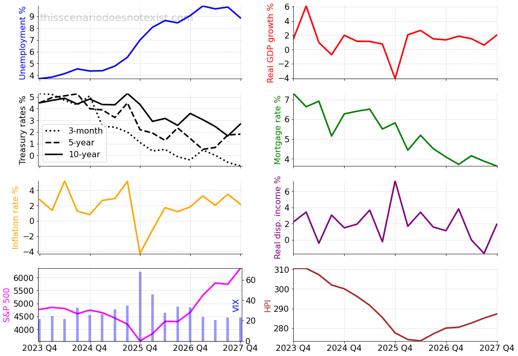
The first economic scenario happens to be a classic recession. Unlike FRB scenarios, the recession does not start immediately from the first quarter of the scenario but rather takes a few periods to develop the right preconditions.

The yield curve stays inverted for a year into the scenario. Then, the 3-month Treasury rate quickly decreases due to less than 2% inflation in the prior two periods and slightly negative GDP. (Note that the 3-month Treasury rate is highly correlated with the Fed Funds rate.) However, the rate cut fails to support job growth as unemployment rises and the increased inflation further weakens the economy.
At the end of the second year, GDP sharply turns negative and the stock market drops 25%, with VIX spiking close to 70. The unemployment rate reaches 7% and continues climbing to 10%. The Treasury 3-month rate continues to decline and even turns negative at the end of the scenario.
Interestingly, real disposable income growth shows an increase at the end of the second year when GDP sharply declines. This phenomenon was observed in historical stress periods as well. The income growth could be a temporary government stimulus or a tax cut, negative inflation (deflation), and wage stickiness as wages take time to adjust.
Home prices started to decline in the early periods of the scenario and slowly recovered in the second half. Overall, home prices fell 12% before the recovery.
Tug-of-war Scenario: Inflation vs Interest Rate
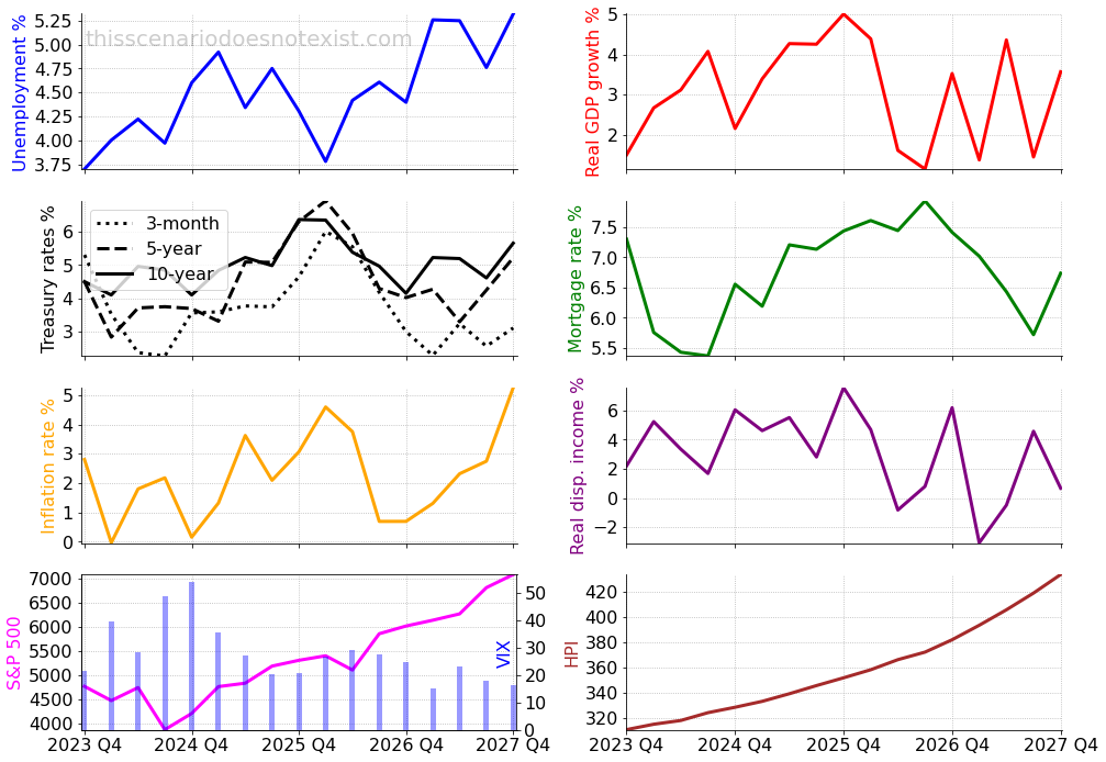
In this economic scenario, the inflation and interest rates seem locked in a tug-of-war. When the inflation rate pushes up, the Treasury 3-month tries to pull it down.

For context, in 2023, the year preceding the scenario, the inflation was trending down and the short-term interest rate increased to over 5%.
At the beginning of this generated economic scenario, the inflation rate goes down, followed by a decrease in the Treasury 3-month rate. Starting from the second year, inflation starts to increase, reaching over 4% at the beginning of the third year. As a response, the Treasury 3-month rate increases to 6%, which helps to slow down inflation significantly.
In the fourth year of the scenario, the inflation rate increases again reaching over 5% at the end of the year. However, this time the Treasury 3-month rate only increases slightly, hovering around 3% due to weakness in the job market.
Real GDP shows a noticeable growth during the first half of the scenario, benefiting from a lower inflation rate and a relatively strong job market. In the second half of the scenario, GDP growth is lower and more volatile impacted by the higher rates and cycling inflation.
The stock market overall gains about 48% during the four years of the scenario. However, it ended lower at the end of the first year due to concerns about an increasing unemployment rate and unstable inflation. VIX is higher during the first half of the scenario reflecting volatile market performance.
Home prices steadily increase, gaining an overall 40% at the end of the scenario. A continuous tight supply and higher construction costs likely drive such an increase in house prices. Besides, elevated investor activity during the fast home price growth period further accelerates the price increase.
Moderate Recession Scenario
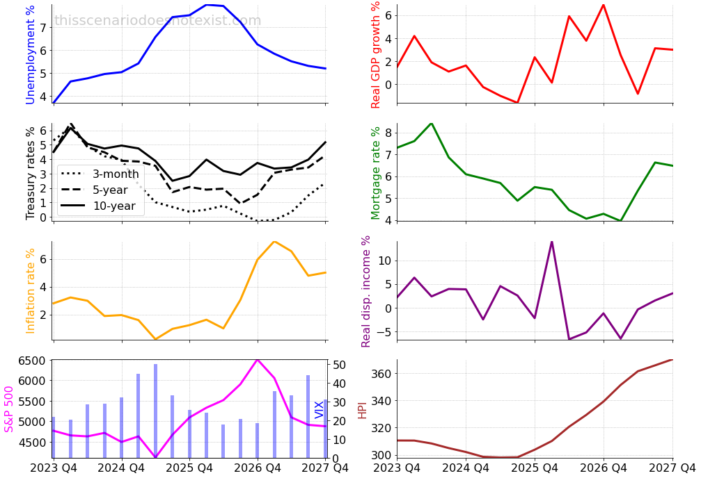
In this economic scenario example, the economy falls into a moderate recession. The unemployment rate increases to 8% and GDP dips into negative territory.

At the beginning of the scenario, the Treasury 3-month rate briefly increases to 6% due to an uptick in inflation. Then, during the following several quarters, the interest rate comes down to a near zero level as inflation slows down and the unemployment rate increases significantly.
At the beginning of the third year, when the unemployment rate reaches 8%, the real disposable income spikes which can be due to government stimulus and tax credits. It helps to recover GDP from the negative growth and reduce the unemployment rate to a 5%-6% level.
However, the quick recovery in the job market and the overstimulated economy (GDP is 4%-6% in the third year) push inflation up. As a result, the Treasury 3-month rate starts to increase to control inflation.
The stock market drops about 14% in the second year due to the developing recession. The increased VIX reflects the uncertainty in the stock market during the period. Then, in anticipation of the economic recovery, the stock market increases by 58% from the drop. However, due to increasing inflation and interest rates in the fourth year, the market loses most of the gain and ends up only at a 2% above the initial level.
House prices experience 4% decrease during the second year compared to the starting level of the scenario. Then, with the economic recovery, the home prices have a 24% trough-to-peak increase. Overall, the home prices have a 19% end-to-end increase in the scenario.
Soft Landing Scenario
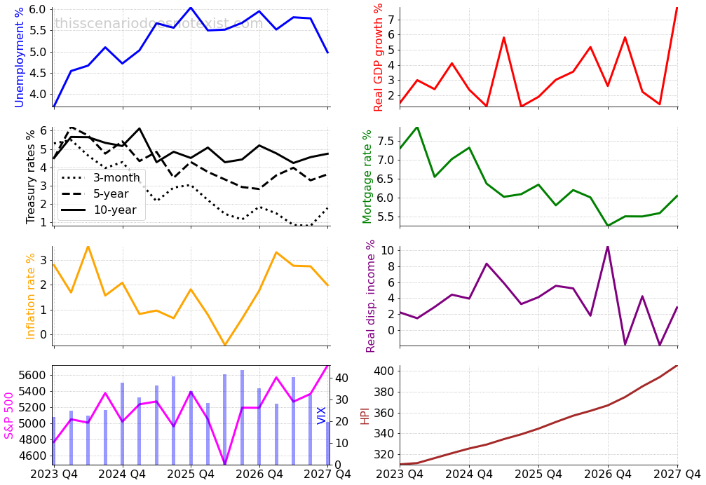
This economic scenario is perhaps close to a soft landing scenario, where inflation is under control and the overall economy performs relatively well. However, from a glass-half-empty view, it may be called a no-landing scenario due to the relatively high unemployment rate and lackluster stock market performance.

The inflation rate mostly stays under 3% and the short-term interest rate is gradually trending down to 1% with some bumps along the way. Real disposable income growth has a couple of spikes, likely the reason for an increase in inflation and GDP in the following periods.
The stock market overall increases by 20% during the four years with a few large and small drops throughout the scenario. VIX is relatively high reaching 40 echoing the stock market’s underperformance.
House prices have a rapid increase, partially driven by higher disposable income and decreasing mortgage rates. Other factors contributing to a total 30% increase in home prices can be population growth, demographic shifts, and, to some degree, speculation, which are not directly reflected in the economic scenario.
Conclusion
The illustrated scenario examples produced by our AI-based economic scenario generator are dynamic and coherent. They maintain a reasonable relationship between macroeconomic variables and adhere to stylized facts such as the relation between inflation and short-term interest rates. The generated scenarios also take into account correlation, lagging effects, and unique patterns observed in stress scenarios.
At Scenarios by AI, we provide simulated economic scenarios that capture the complex dynamics of macroeconomic indicators. Reach out to explore how these generated economic scenarios can help you enhance your portfolio risk management.
