
One important feature of the Economic Scenario Generators (ESG) is the reproduction of stylized facts observed in the historical data. While it might be challenging to quantify all stylized facts, a simple comparison of correlations between the historical data and the generated scenarios can provide significant insights into the behaviour of economic variables.
We use our AI-based economic scenario generator (ESG) to generate hundreds of economic scenarios. All generated scenarios are based on the Q4 2024 starting point and cover 48 quarters (12 years). The scenarios have 12 macroeconomic variables:
- Inflation rate
- Unemployment rate
- Treasury 3-month rate
- Treasury 5-year rate
- Treasury 10-year rate
- Mortgage rate
- Real disposable income growth
- Real GDP growth
- VIX (maximum close-of-day value in a quarter)
- S&P 500 growth
- HPI growth
- WTI (oil price)
We calculated correlations between economic variables in the generated scenarios and compared them with the historical correlations. We used Spearman correlation (instead of Pearson correlation) to avoid the impact of outliers. Note that we also calculated the Pearson correlations, which were very close to the Spearman correlations in generated scenarios.
Correlations in Generated Economic Scenarios
For each scenario, we calculated the pairwise correlations between 12 economic variables. This resulted in a 12 by 12 correlation matrix. Then we calculated the average correlation matrix across all generated scenarios. Note that all generated economic scenarios are independent of each other and are conditional on the starting point, which is Q4 2024.
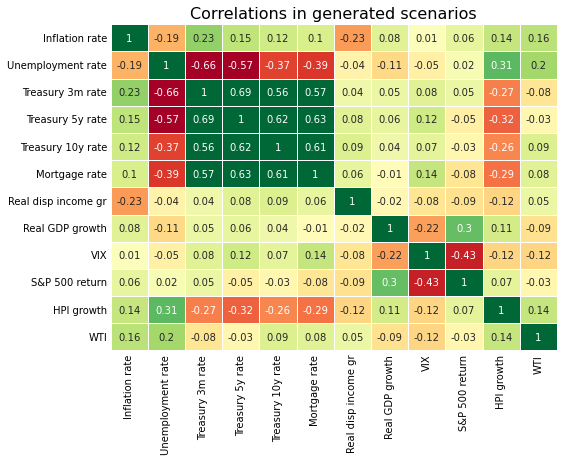
We can observe strong positive correlations between interest rates. Besides, the interest rates are positively correlated with the inflation rate. It makes sense since usually the interest rates increase in response to rising inflation, then decrease when the inflation falls.
On the other hand, the interest rates are negatively correlated with the unemployment rate, since the Fed usually cuts the interest rate when the unemployment is elevated.
Other notable correlations are a strong negative relationship between S&P 500 return and VIX, a positive relation between inflation rate and oil price (WTI), and a negative correlation between interest rates and house price (HPI) growth.
One counterintuitive relation is the positive correlation between HPI growth and unemployment rate. One would expect declining house prices in an economy with increasing unemployment. To gain insight into this phenomenon, let’s look at the correlations between economic variables in the historical data.
Historical Correlations between Economic Variables
Unlike generated scenarios, which can be in hundreds or even thousands, there is only one historical economic scenario. This presents a challenge for comparing historical correlations with the generated ones.
To be relatively consistent with the correlation methodology for generated scenarios, we used a 48-quarter rolling window to calculate the historical correlations. For each window, we calculated the correlation matrix, then averaged out across all windows.
We must recognize that the historical scenarios in the 48-quarter rolling windows are not independent, as they can overlap. In contrast, the generated scenarios are independent after accounting for being conditioned on the same starting point. In an attempt to mimic the methodology of the correlation calculations for the generated scenarios, we also calculated the average historical correlations with non-overlapping 48-quarter windows. The resulting correlation matrix was very close to the one obtained with the rolling window approach. We chose to use the rolling window approach as it is based on a larger sample (although not independent).
Another challenge with the historical 48-quarter scenarios is that they are based on different starting points, while the generated scenarios are conditional on the initial point. With all these differences in mind, we calculated the correlations between economic variables in the historical data.
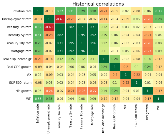
Most of the correlations in the historical data are similar to the ones in the generated scenarios. For example, strong positive correlations between interest rates, a positive correlation between interest rates and inflation rate, and a negative correlation between S&P 500 return and VIX.
However, the historical data shows a negative correlation between the unemployment rate and HPI growth. This appears more intuitive as in the weakening economy with increasing unemployment, the housing demand generally declines while the supply increases, leading to a decline in house prices.
Correlation between Unemployment Rate and HPI Growth
To better understand the discrepancy of this correlation between historical and generated scenarios, we took a closer look at the historical data. Specifically, we analyzed the dynamics of the historical correlation between the unemployment rate and HPI growth.
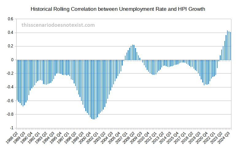
The time series on the chart represents correlation produced by a 48-quarter sliding window. At each point, the value of the time series is the Spearman correlation between the unemployment rate and HPI growth for the 48 quarters ending at the point.
While most of the time the correlation was negative, it turned positive starting from 2022. Interestingly, the last time we observed a positive correlation between unemployment rate and HPI growth was during the financial crisis in 2007-2009.
One of the economic factors contributing to the positive correlation starting from 2022 is the limited housing supply. Additionally, post-pandemic low interest rates and increased inflation further contributed to the increase in house prices. On the other hand, the increased unemployment during the pandemic period did not negatively impact the housing prices, as the layoffs were concentrated in selected labor market sectors. This structural change in the labor market resulted in the departure from historical patterns where the relationship between the unemployment rate and HPI growth was negative.
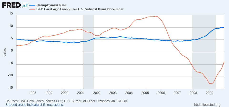
The positive correlation in 2007-2009 was driven by different factors. HPI growth was a leading indicator for the Great Recession. It started to decline in the second half of 2005 when the unemployment rate was still declining. Besides, HPI growth bottomed in early 2009 when the unemployment rate was still rising (notice, this is HPI growth and not HPI level).
As a result, the 12-year sliding window correlation between the unemployment rate and HPI growth turned positive in 2007-2009.
Since most of the time the historical correlation was negative, it resulted in an overall negative correlation between the unemployment rate and HPI growth in the historical correlation matrix. On the other hand, the generated scenarios are conditional on the starting point where the correlation is positive. This positive relation has been carried forward in many generated scenarios, resulting in an overall positive correlation between the unemployment rate and HPI growth.
Summary
Analysing the correlations between economic variables in the generated scenarios is a simple way of assuring the quality and consistency of the scenarios. We have seen that most of the correlations are consistent with the correlations observed in the historical data. We noted a departure from the historical relation for the correlation between the unemployment rate and HPI growth. This discrepancy is attributed mainly to the starting point of the generated scenarios, where this correlation has been positive starting from 2022.